Benchmark: Chebyshev vs. Direct Solvers

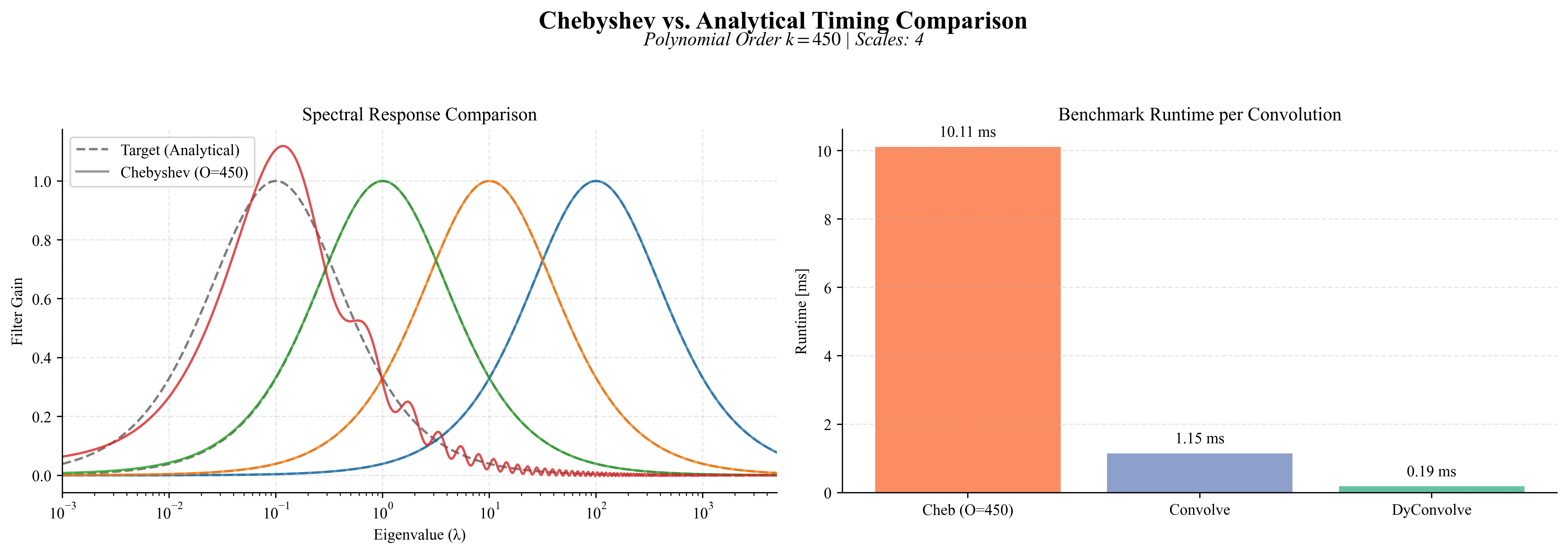
This benchmark demonstrates the performance trade-offs between polynomial approximation and sparse direct solvers. In most cases, the optimized DyConvolve solver outperforms high-order Chebyshev approximations on large sparse graphs.

Chebyshev vs. Analytical Timing

SCALES = [0.01, 0.1, 1, 10]
ORDER = 450
N_ITER = 200
X = impulse(L, n=1200)

def f(x): return np.stack([sgwt.functions.bandpass(x, scale=s, order=1) for s in SCALES], axis=1)

lbnd = 1e-3
kernel = sgwt.ChebyKernel.from_function_on_graph(L, f, ORDER, min_lambda=lbnd)

print(f"Benchmarking on {L.shape[0]} nodes...")

# Time Chebyshev Convolution
with ChebyConvolve(L) as conv_cheb:
    _ = conv_cheb.convolve(X, kernel)
    start = time.time()
    for _ in range(N_ITER):
        _ = conv_cheb.convolve(X, kernel)
    t_cheb = (time.time() - start) / N_ITER

# Time DyConvolve, which pre-factors to time only the solve phase.
with DyConvolve(L, poles=[1.0/s for s in SCALES]) as conv_dy:
    _ = conv_dy.bandpass(X)
    start = time.time()
    for _ in range(N_ITER):
        _ = conv_dy.bandpass(X)
    t_analytical = (time.time() - start) / N_ITER

# Time Convolve, which includes factorization in each call.
with Convolve(L) as conv_std:
    _ = conv_std.bandpass(X, SCALES)
    start = time.time()
    for _ in range(N_ITER):
        _ = conv_std.bandpass(X, SCALES)
    t_std = (time.time() - start) / N_ITER

print(f"Chebyshev (Order {ORDER}): {t_cheb*1000:.2f} ms")
print(f"Convolve:  {t_std*1000:.2f} ms")
print(f"DyConvolve:  {t_analytical*1000:.2f} ms")