Local Mode Identification
Demonstrates computing the SGMA spectrum at a single bus to identify dominant oscillatory modes in the wavelength-frequency domain.
The Joint Spectrum
For a target bus \(n\) and time \(\tau\), the SGMA computes the joint wavelet transform:
The resulting spectrum \(m_{n,\tau}\) reveals the energy distribution across spatial wavelengths (related to \(\sqrt{s}\)) and temporal frequencies. Peaks in this 2D spectrum correspond to dominant oscillatory modes.
This example shows how to:
Initialize the
SGMAengine with spatial scales and temporal frequencies.Compute the spectrum for a specific bus and time using
sgma.spectrum().Extract modes with
sgma.find_modes()to obtain frequency, damping, and wavelength.
from sgwt import SGMA
from sgwt import LENGTH_WECC as L

# Signals: Real or Complex Matrix (Rows: Buses, Cols: Time)
V, t = get_signal(FILEPATH, t_range=(0, 60))

# SGMA Parameters
BUS_TARGET = 36
TIME_TARGET = 2.0
ORDER = 1
TOP_N = 3

wmin = 1
wmax = 3e3
nscales = 150
spatial_scales = np.geomspace(wmin**2, wmax**2, nscales)

temporal_freqs = np.linspace(0.05, 2.0, 100)
sgma = SGMA(L, spatial_scales, temporal_freqs, order=ORDER, w0=2*np.pi)

# Get complex spectrum (compute once)
M = sgma.spectrum(V, t, BUS_TARGET, TIME_TARGET, return_complex=True)

# Identify modes with frequency, damping ratio, wavelength, and magnitude
modes = sgma.find_modes(M, top_n=TOP_N)
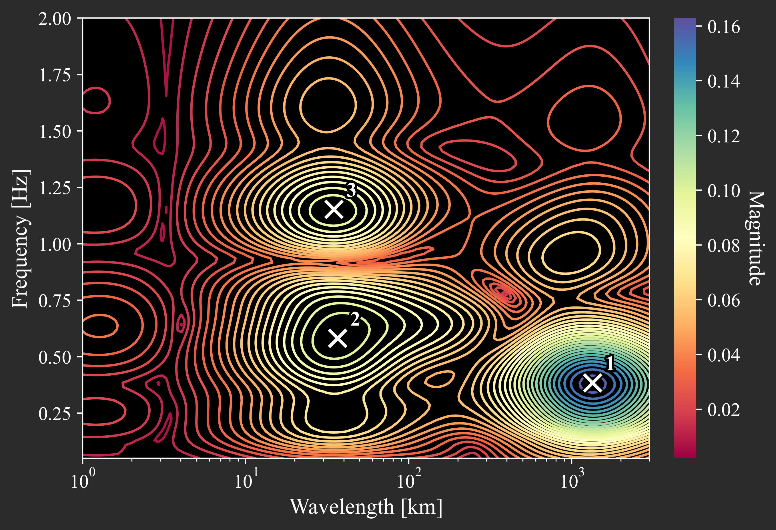
The contour plot shows the spectrum magnitude in the wavelength-frequency domain.
The overlaid markers indicate the top_n most dominant oscillatory modes (peaks)
identified at the target bus and time instant. Each peak provides:
Wavelength \(r = \sqrt{s}\): spatial extent of the mode
Frequency \(f_0\): oscillation rate in Hz
Damping \(\zeta\): decay rate estimated from phase slope
IEEE 39 Bus New England Case
The IEEE 39 bus New England ISO case demonstrates SGMA on a real-world power system topology. The signal is the complex voltage response to a balanced three-phase fault at Bus 16, occurring at \(t=0.5\) seconds and cleared at \(t=0.7\) seconds. The simulation uses a time step of 1 millisecond from \(t=0\) to \(t=10\) seconds.
SGMA Parameters
The analysis uses the following configuration:
- Graph and Analysis Point:
Laplacian:
LENGTH_NEISO(39 buses)Target bus: 12
Target time: \(\tau = 1.5\) seconds
Bandpass order: \(K = 1\)
- Spatial Sampling:
Number of scales: 150
Scale range: \(s \in [(0.1)^2, (100)^2]\) (geometrically spaced)
Wavelength range: \(r = \sqrt{s} \in [0.1, 100.0]\)
- Temporal Sampling:
Number of frequencies: 200
Frequency range: \(f \in [0.01, 3.0]\) Hz (linearly spaced)
Wavelet parameter: \(\omega_0 = 2\pi\)
from sgwt import SGMA
from sgwt import LENGTH_NEISO as L

# Signals: Real or Complex Matrix (Rows: Buses, Cols: Time)
V, t = get_signal(FILEPATH)

# SGMA Parameters
BUS_TARGET = 12
TIME_TARGET = 1.5
ORDER = 1
TOP_N = 3

wmin = 1e-1#1
wmax = 1e2#3e3
nscales = 150
spatial_scales = np.geomspace(wmin**2, wmax**2, nscales)

temporal_freqs = np.linspace(0.01, 3, 200)
sgma = SGMA(L, spatial_scales, temporal_freqs, order=ORDER, w0=2*np.pi)

# Get complex spectrum (compute once)
M = sgma.spectrum(V, t, BUS_TARGET, TIME_TARGET, return_complex=True)

# Identify modes with frequency, damping ratio, wavelength, and magnitude
modes = sgma.find_modes(M, top_n=TOP_N)
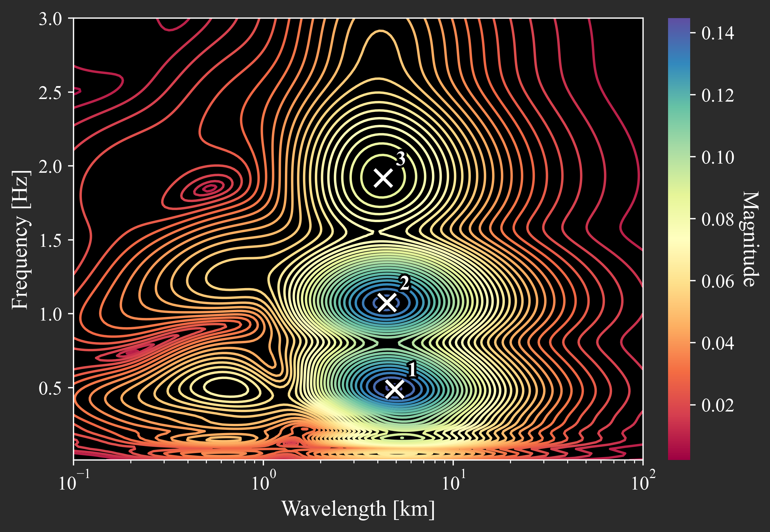
Identified Modes
The find_modes function extracts the top 3 peaks from the spectrum:
------------------------------------------------------------
#   Freq (Hz)     Damping    Wavelength   Magnitude
------------------------------------------------------------
1      0.4908      0.0000          4.91      0.0209
2      1.0768      0.3920          4.48      0.0201
3      1.9182      0.1638          4.27      0.0084
------------------------------------------------------------
- Each mode is characterized by:
Frequency (Hz): Oscillation rate extracted from the temporal frequency axis
Damping: Decay rate estimated from phase variation in the complex spectrum
Wavelength: \(r = \sqrt{s}\) at the peak location in the spatial domain
Magnitude: Transform magnitude at the peak location